Using deep learning to undo line anti-aliasing

What is the problem?

DaltonLens is a desktop utility I developed to help people with color vision deficiencies, and in particular to parse color-coded charts and plots. Its main feature is to let the user click on a color, and highlight all the other parts of the image with the same color. Below is a video illustrating the feature:

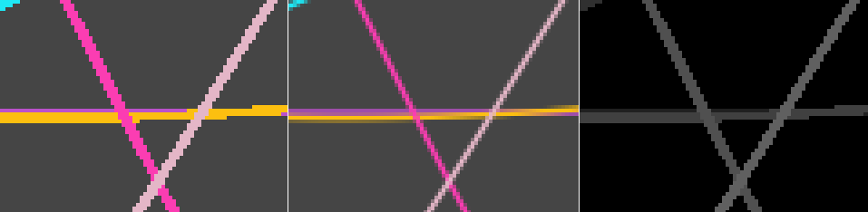
This is trivial to implement for constant color areas, but for thin lines, small markers or text it actually gets more complicated, especially if the background is not uniform. The reason is anti-aliasing. To get nice-looking lines, the foreground stroke path gets blended with the background when pixels are only partially filled. This creates a set of intermediate colors instead of a flat constant color. Here is how an anti-aliased line looks like once zoomed in:

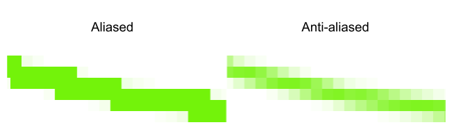
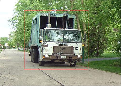
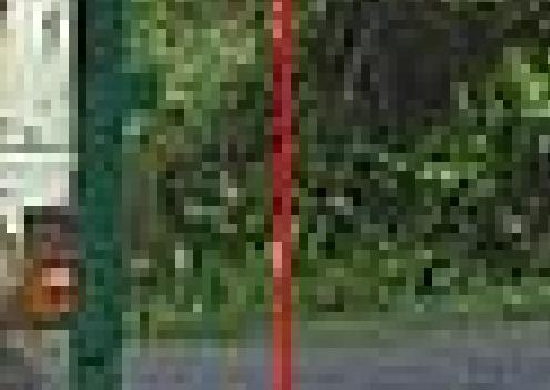
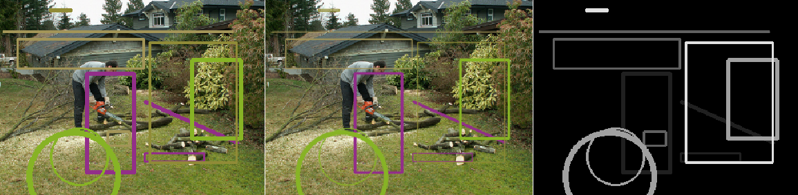
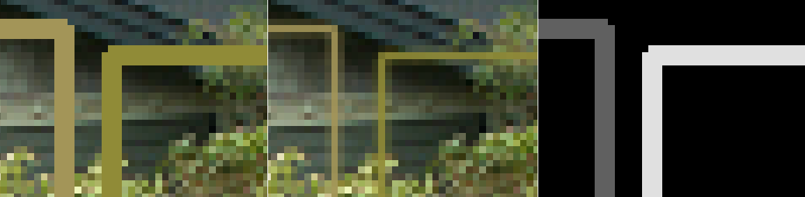
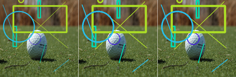
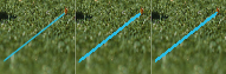
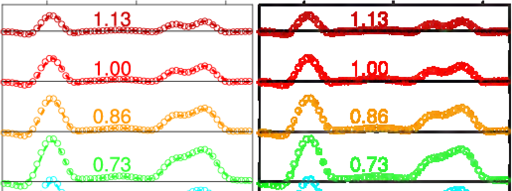
The aliased image is trivial to segment, but as you can see the colors are no longer constant in the anti-aliased one. In fact, the exact original solid line color may not appear at all in the anti-aliased rendering if the stroke width is less than 1 pixel. To workaround this DaltonLens implements a smarter thresholding in the HSV space that gives more importance to the hue and less importance to saturation and value. This works reasonably well when the background is uniform, but when the stroke is really thin or the background more complex it tends to fail and only highlight a small portion of the foreground objects. Below is a difficult case where a color annotation was added on top of a natural image. The right image zooms on a rectangle segment in the right side.

Unfortunately these hard cases are also the ones where an assistive tool is most useful for someone with a color vision deficiency. Fundamentally the problem is hard to solve at the pixel level, and it requires a larger context to group the colored pixels together and figure out that even if their RGB values don’t exactly match, these patterns still belong to the same object.

To address this, one option is to keep adding better heuristics, trying to group pixels with more elaborate segmentation methods, for example graph-cuts or other energy-based methods. These can try to balance some color similarity measure with a regularization term encoding our prior knowledge about the image content.

As an example the approach of Antialiasing Recovery by Yang et al. works pretty well when one can assume that the edges fundamentally have two single dominant colors on each side. But this is not the case when a natural background is used, for example when annotating a picture with labels. It also won’t work very well for structures that are thinner than 1 pixels since the actual original object color may not appear at all in the neighborhood.

Approching the problem with deep learning

Observing that it’s quite easy to generate anti-aliased plots with a ground truth foreground color, it’s tempting to try a deep learning based approach instead of building more complex heuristics. If the learned model fails in some images, we can always add more examples of similar cases to improve it.

So I’ve decided to give it a try as part of my journey to catch up with deep learning for computer vision.

Generating ground truth data

As a first step I’ve generated images with OpenCV line, rectangle and circle primitives on top of a uniform colored background. Some parameters are sampled randomly:

• The start/end/radius of the primitives
• The stroke width
• The foreground and background colors, ensuring that they are all significantly different.

Then the primitives are rendered using cv2.LINE_AA. The source code is available on github.

To generate the ground truth, the simplest option would have been to render the same primitives without cv2.LINE_AA. But instead I’ve decided to make it so any pixel that was touched by the primitive should be filled, so that the resulting paths get thicker and thus easier to visualize and more obvious once highlighted. This can be done by rendering the primitives one by one over a uniform background and computing the mask of the pixels that changed.

Finally the ground truth data for one image is simply a pair of images: the rendered anti-aliased image (the input) and the corresponding aliased image with solid colors (the target output). In addition an image of labels (between 0 and 255) gets generated along with a json file that associate each label to an RGB color. It is somewhat redundant with the target aliased image, but having this information can be useful to implement smarter loss functions (e.g. ensuring that the output color is very constant for a given label is more important for my application than the actual absolute value).

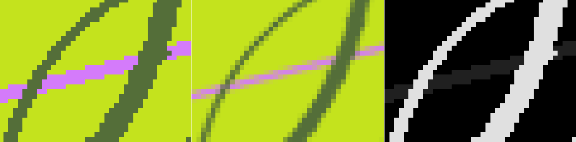
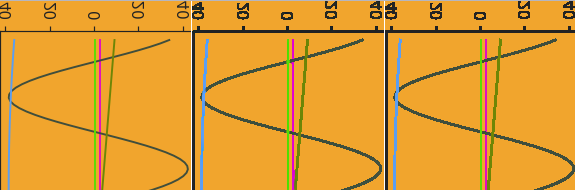
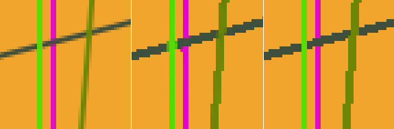
Here is a generated sample (aliased, anti-aliased and labels) and a zoomed area.

In addition to this I’ve generated images with a natural background too. I used imagenette2 to randomly sample a background, and then draw the primitives on top of it. The aliased image does not change the pixels of the background since only the foreground paths are anti-aliased.

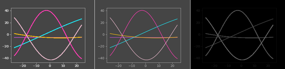
Finally I generated plot and scatter images in a similar way with matplotlib, this time picking functions and their parameters randomly, in addition to their colors and stroke width.

Overall I generated ~5000 images from each category.

Training a baseline model

Now that we have some training data, let’s see if we can train a model to output an aliased image from the input anti-aliased image. For this kind of image to image problem, I first chose a straightforward approach:

• Input is the anti-aliased image in RGB, normalized to a mean of 0 and deviation of 1.
• L2 loss between the RGB values of the output image and the target aliased image (also normalized).
• Inspired by fast.ai dynamic UNet, I picked a UNet architecture, with a pre-trained Resnet18 encoder.
• The data is augmented with random crops locations and vertical / horizontal flips to avoid overfitting to specific locations.

Trained for a hundred epochs, it gives pretty good results on unseen images that were generated by the same procedure.

This loss has a number of problems though:

• L2 is known to favor a blurry output. And it’s quite sensitive to mispredictions of the aliased mask. It’s easy to miss pixels that were very partially filled, and thus the network tends to favor blurry solutions that keep some of the background in complex areas instead of picking a clear solid color.

• The network spends a lot of energy learning how to reconstruct the background pixels, which actually didn’t change at all. Making the UNet output become additive to the original image helps, but is still suboptimal.

• In our case we don’t care as much about finding the exact original solid color, what matters more is that the reconstructed pixels belonging to the same object all share the same solid color so we can segment them easily afterwards.

Refining the model with a gated output

To address some of these shortcomings, I tried to separate the problem of detecting what pixels belong to an anti-aliased primitive from the problem of assigning a solid color to that primitive.

A simple way of doing that is to have the model also output a binary mask, 0 if it’s background, 1 if it’s an anti-aliased primitive. Then I made the loss become a combination of losses:

1. A binary cross-entropy loss for the fg/bg mask. The ground truth foreground mask is easy to extact from the labels image (anything not zero).
2. An L2 loss for the pixels considered as foreground by both the target output and the model. This way it will only penalize foreground pixels that don’t have the right color, but ignore the color of pixels that were classified as foreground instead of background. This way the network does not have to be conservative and stay too close to the original image.
3. I also optionally added a third loss that computes the variance of the output foreground pixels for a single foreground label, picked randomly. The idea was to enforce a constant color output for each label, accepting a small bias from the true absolute color. In practice it did not really bring an improvement, more investigation would be needed on that.

The final output image can be computed as a composite of the unchanged input image (when mask < 0.5) and the rgb output (when mask > 0.5). This “gated” approach makes the training easier and spend much less time learning to reconstruct background pixels properly.

It’s worth noting a small extra refinement too, I added a small encoder at the full-resolution image since that’s where most of the anti-aliasing information is. Here is a diagram of the implemented network.

And some results.

Extending the training set with arXiv figures

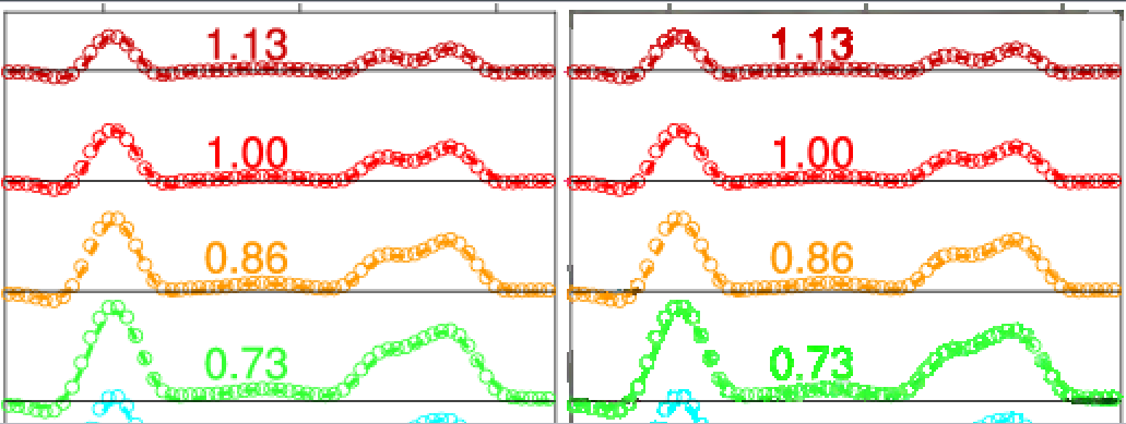
These results are pretty encouraging and show that the network is able to reconstruct anti-aliased primitives even on images with a natural background. But it does not work as well on plot images taken from the wild. Here is an example where the model basically leaves the input unchanged, because it never saw that kind of patterns before:

The main problem is that our generated images are not representative enough of the large variety of plots and charts that can be found in the wild. Unfortunately it is hard to find large datasets of plots and charts from which we can extract ground truth aliased image. The best source I found is arXiv, which publishes its database of paper, including the sources, as S3 buckets. And in the sources we can often find PDF files of the figures. And since PDF plots are vectorial drawings, it becomes possible to render them with and without anti-aliasing to generate ground truth data.

There are a number of practical difficulties to extract a meaningful set of figures from the raw paper sources, but I was able to build a reasonable pipeline and extract ~1000 images from a fraction of the March 2022 archives alone. The source code is available here. My main steps are:

• Use PyMuPDF to check each pdf file and determine whether it has enough colors, a reasonable complexity, image size, etc.

• Then convert the PDF to SVG with CairoSVG, converting text to paths along the way to avoid font issues.

• Modify the SVG file to make sure that the stroke width is always at least 2. Otherwise the aliased rendering might be very thin.

• Optionally modify the SVG to add a different background color as most figures otherwise have a white background.

• Convert the modified SVG back to PDF and render it with ghostscript with anti-aliasing disabled.

• Also check which pixels changed between the antialiased and aliased rendering to build the ground truth mask.

This pipeline is fully automated, but some figures are not great and the computed ground truth is not always perfect. So I combined this process with an interactive viewing tool (based on my zv image viewer) to quickly validate or discard the generated samples. Below is an example of arXiv training sample.

After adding that kind of data, the results are now better on some images. Here is what we get on the image we tested earlier, this time it managed to make it aliased with solid colors again:

What’s next?

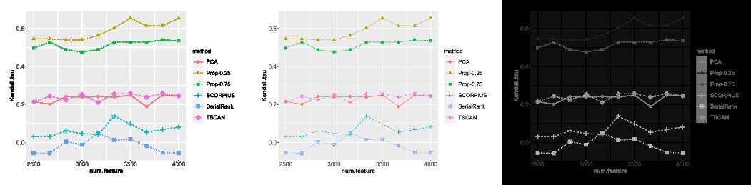
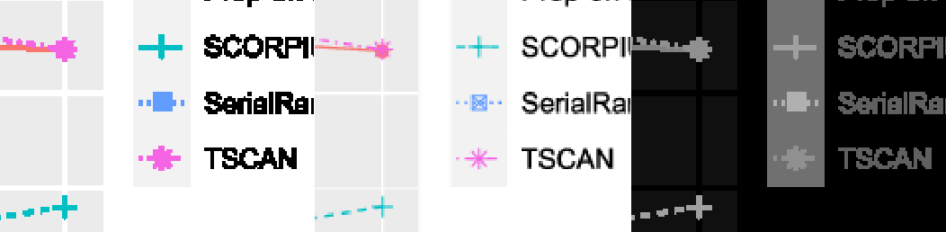
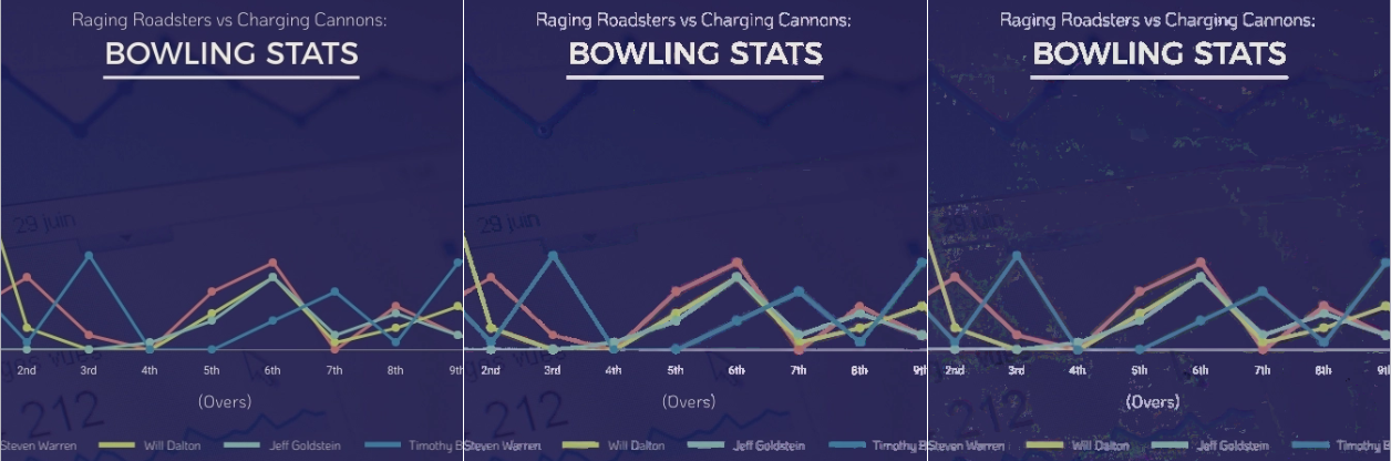
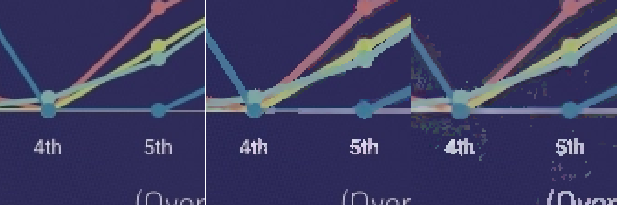
Even with the arXiv dataset we still lack a representative training set for “designer” charts that can be typically found in e.g online newspapers. These tend to have fancier backgrounds and paths than arXiv papers. Here is an example where the model still struggles, and actually got worse after including the arXiv datasets:

So overall we’ve transformed the problem of handcrafting color segmentation algorithms into a problem of collecting or generating good enough data. Besides collecting more data, there are a number of improvements that seem worth investigating:

• The loss function is still not great. The variance term did not really help to to favor outputs that have a very solid color, downplaying the importance of matching the exact foreground mask. One idea there is to learn the loss by training the network in a GAN setup. I quickly tried a vanilla Pix2Pix and got poor results, but the “no-GAN” setup of https://github.com/jantic/DeOldify sounds appealing as a final step.

• Transformers may also be a better fit for this problem as they could use a global context to infer the small set of solid colors and spread them everywhere. Approaches like Restormer (CVPR2022) look promising.

• It could also be interesting to take a completely different approach and formulate the problem as an object detection one, with the classes being quantized colors. Something like DETR, which was tuned for line segmentation in LETR (Line Segment Detection Using Transformers without Edges). This would inject the prior that there are only stroke paths with a few distinct colors to find in the input image.

Resources

• It’s a mess at this stage, but here is the repository with the source code to generate images, etc.: DaltonLens/DaltonLens-Research .

• Online demo on HuggingFace spaces